3D Reconstruction of Potted Cotton by Turntable Photogrammetry

Overview

Single-plant 3D models are the input to organ-level phenotyping and to canopy light and photosynthesis simulation. This protocol reconstructs potted cotton plants in a growth chamber by turntable photogrammetry: the plant rotates in front of two fixed cameras at different elevations, and structure from motion (SfM) turns the image sequence into a scaled point cloud and mesh.

The protocol has three aims:

• a standardized multi-view image dataset for each plant;
• a metric 3D reconstruction for plant architecture analysis and light-distribution modelling;
• quantified reconstruction accuracy and colour consistency.

1. Imaging environment

• Chamber. A growth chamber with controlled temperature, humidity and light. Fans are stopped during capture, because small leaf movements break feature matching between views.
• Light. Uniform diffuse light of 500–800 lx from side-mounted diffusing LED panels; ceiling spotlights are switched off to avoid specular highlights and hard shadows.
• Background. Black non-reflective cloth over background and floor, which suppresses reflections and makes masking simple.
• Turntable. An acrylic turntable 60–80 cm in diameter, covered with diffusing film to remove specular reflection, motor-driven at constant speed with one revolution in 60–90 s. The pot is centred on the rotation axis and stabilized if needed.
• Scale and control. Coded markers and measured scale bars are fixed on the turntable, so they rotate with the plant. Marker layouts avoid symmetry, which can produce ambiguous correspondences. One measured distance is kept out of the scaling and used as an independent check.
• Colour. A SpyderCheckr 24 chart is placed in the field of view of both cameras to monitor and correct colour.

In turntable capture the plant moves relative to the room, so everything static (background, colour chart, supports) is masked out of the reconstruction.

2. Cameras

	Camera A	Camera B
Device	iPhone Pro (13 Pro or later)	iPhone Pro (13 Pro or later)
Elevation	−45° (looking down)	0° (horizontal)
Distance	≈ 1.0 m	≈ 1.2 m
Recording	4K (3840 × 2160), 30 fps	4K (3840 × 2160), 30 fps

Focus, exposure, white balance and focal length are locked on both cameras; automatic HDR and lens switching are disabled. The two elevations cover the upper surfaces and the sides of the plant and reduce occlusion between leaf layers. Device, lens, resolution and exposure settings are recorded with each session.

3. Capture

1. Centre and secure the pot without touching the leaves; record plant ID, treatment and date.
2. Start the turntable and let it reach constant speed.
3. Start recording on both cameras.
4. Record one full revolution, checking that the plant, markers and chart stay in frame.
5. Stop recording and name the files by plant, camera and elevation, e.g. Plant01_A_45.mp4, Plant01_B_0.mp4.
6. Review the sequence for blur, exposure drift and leaf movement before removing the plant.

4. Pre-processing

Colour correction. In DaVinci Resolve, colour balance is calibrated against the SpyderCheckr 24 chart, and the same correction is applied to the whole sequence. The uncorrected videos and the correction parameters are kept. Colour correction makes images consistent across plants and sessions; it does not convert pixel values to reflectance.

Frame selection. A 4K, 30 fps revolution of 60–90 s gives 1,800–2,700 frames per camera, most of them nearly identical. Frames are therefore thinned to an even angular spacing that keeps strong overlap between neighbouring views, and blurred frames are discarded. The final angular interval, number of retained frames and rejection reasons are recorded.

File organization.

Plant01/
├── raw_videos/        # Plant01_A_45.mp4, Plant01_B_0.mp4
├── frames/
│   ├── A_45/          # Plant01_A_45_0001.jpg …
│   └── B_0/
├── masks/
├── calibration/       # colour chart, scale bars, camera settings
├── metashape/         # Plant01.psx and exports
└── validation/        # manual measurements

5. Reconstruction in Agisoft Metashape

1. Import the frames as two camera groups (A −45°, B 0°) and apply masks.
2. Align Photos at high accuracy with generic preselection (starting values: key-point limit 40,000, tie-point limit 10,000), then inspect the sparse cloud and remove clear outlier tie points.
3. Detect the coded markers, enter the measured scale-bar distances and run Optimize Cameras.
4. Build Dense Cloud at high quality with mild depth filtering, which preserves thin leaf margins.
5. Remove remaining background geometry, then Build Mesh from the dense cloud and, when needed, Build Texture (generic mapping, mosaic blending).
6. Export the point cloud or mesh (PLY, OBJ or GLB) in metres, with camera positions.

Point clouds are cleaned and organ-labelled in CloudCompare or Open3D. The figure below is a result of this protocol: cotton sample 20240109-84-5 reconstructed by SfM, with points labelled as main stem, branches and petioles, or leaves.

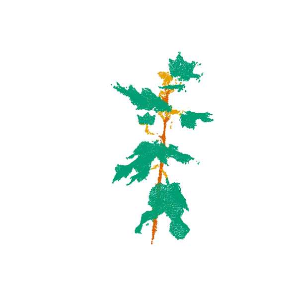
Interactive SfM point cloud of a cotton plant

Sample cotton_20240109-84-5, reconstructed with structure from motion: all 39,765 points, coloured by organ class.

6. Accuracy assessment

Each reconstruction is reported with:

• the number of input and aligned images;
• camera reprojection error;
• marker and scale-bar residuals;
• the error on the independent check distance;
• regions that are visibly missing or falsely filled.

Plant height and canopy width measured by hand (m_i) are compared with the reconstructed values (r_i):

bias = mean(r_i − m_i)
RMSE = sqrt(mean((r_i − m_i)²))

Repeated captures of the same plants give the repeatability of each trait. Colour correction is checked by comparing the corrected chart patches with their reference values.

7. Trait extraction and data products

Plant height, canopy width, volume and leaf inclination are extracted with Python, Open3D and NumPy. Each plant's record keeps the raw videos, selected-frame list, masks, calibration records, Metashape project and software version, scale constraints, validation measurements, exported models in metric units, and the scripts and parameters used for trait extraction. The organ-labelled point clouds are the input to the triangle-facet canopy used in the canopy photosynthesis model.

Scope and limitations

Turntable photogrammetry assumes a rigid plant: leaf movement during rotation, thin leaf margins, overlapping leaves and texture-poor surfaces are the main sources of missing or false geometry. The protocol suits potted plants up to about the turntable diameter; larger plants and field canopies need a moving-camera or UAV acquisition.