UAV 3D Crop Phenotyping: Cross-Circular Oblique Acquisition, SfM and CanopyPC

Overview

Plot-level 3D structure (canopy height, volume, vertical distribution, row geometry) carries information about growth, lodging risk and light interception that 2D vegetation indices miss. Standard nadir mapping flights are designed for orthomosaics and see mostly the canopy top, so the reconstructed 3D structure is incomplete.

This workflow is built for 3D. It uses a Cross-Circular Oblique (CCO) flight design that views the canopy from many azimuths, reconstructs the field with Structure from Motion (SfM), extracts plot-level 3D traits with the point-cloud tool CanopyPC, and links those traits to crop traits with machine learning.

Workflow

1. CCO flight design

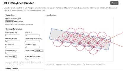
CCO flies sets of circular oblique paths in crossing directions over the field. Each canopy point is seen from many azimuths and two or more view angles, which strengthens the geometric constraints of SfM and fills in canopy sides that nadir flights miss. An additional grid flight provides uniform coverage for the orthomosaic. Forward and side overlap are set higher than for orthomosaic mapping, because the goal is 3D reconstruction rather than a 2D mosaic.

Flight altitude, circle radius, camera pitch and overlap are chosen from the required ground sampling distance, the canopy height and the smallest structure that must be resolved, and are tested on a pilot block before a campaign. Scale and geo-reference come from ground control points (GCPs) or RTK/PPK positioning.

The browser-based CCO Waylines Builder turns a KML field boundary into DJI-compatible KML, WPML and KMZ mission files; the tutorial explains its use.

2. Image acquisition

Images are captured with locked exposure and focus, and a shutter speed short enough to freeze both aircraft motion and leaf motion. Flights are scheduled in low wind and stable illumination, and representative images are checked at full resolution before leaving the field. Aircraft, camera, mission geometry, coordinate system, weather and timestamps are recorded with every flight.

3. Spatial reference: orthomosaic, DSM and point cloud

Alignment of the multi-view images gives camera poses, a dense point cloud, a digital surface model (DSM) and an orthomosaic. The orthomosaic provides the 2D spatial reference: plot boundaries, labels and the coordinate frame to which the 3D results are aligned. The point cloud and DSM carry the 3D structure.

4. Field and plot boundaries

Field boundaries are extracted from the orthomosaic:

1. vegetation indices and texture separate crop from non-crop areas;
2. morphological operations and region growing remove roads, bare soil and border effects;
3. contour extraction and polygon fitting give closed plot polygons.

Plot polygons, combined with the experimental layout, are used to crop the point cloud plot by plot. The Land Surveyor records and exports field polygons on site.

5. 3D reconstruction

SfM point cloud. SfM reconstruction gives the canopy point cloud used for all metric traits: height distribution, spatial heterogeneity and structure at population scale. Reconstructions are checked for GCP/RTK residuals on independent checkpoints, reprojection error, holes under dense upper foliage, floating points and consistency of registration across dates. With CCO acquisition the reconstruction reaches centimetre-level accuracy.

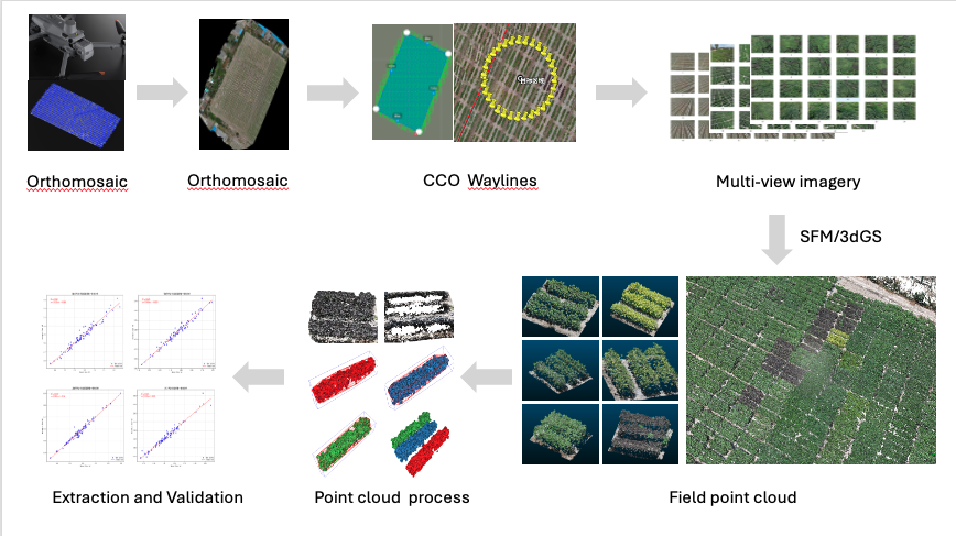
3D Gaussian Splatting. On top of the SfM camera poses, 3DGS gives a continuous, high-fidelity representation of the canopy for interactive 3D inspection of fine structures such as leaf–branch intersections. Metric traits are computed from the SfM point cloud; geometry extracted from 3DGS is validated separately before being used for measurement.

6. CanopyPC: canopy point-cloud processing

CanopyPC is a Python tool I developed for processing CCO-reconstructed canopy point clouds:

• Ground–canopy separation with the Cloth Simulation Filter (CSF); canopy height is measured relative to the filtered ground, not from absolute elevation.
• Pre-processing: statistical outlier removal, removal of small clusters with DBSCAN, removal of ground-control markers, and manual selection for remaining artefacts.
• Row segmentation with K-means clustering.
• Geometry: convex-hull volume, oriented bounding box, projected area and plant-height statistics.
• Visualization of point clouds, hulls and bounding boxes for interactive inspection.

7. 3D structural traits

For each plot or row:

• height statistics: mean, variance and percentiles (e.g. H50, H90, H99), which are robust to single noisy points;
• vertical profile of point density;
• projected canopy area, convex-hull volume and oriented bounding box;
• spatial heterogeneity and aggregation of points;
• canopy surface roughness and undulation;
• row width and gaps.

8. Machine-learning models

3D traits are combined into multi-scale features and linked to crop traits such as biomass, leaf area index or yield with random forest, gradient boosting and related regressors. Validation keeps related samples together: plots, sites and dates are grouped so that the test set contains no plots or flights seen in training. Results are reported per crop, growth stage and site, with error metrics in physical units and comparison to a simple baseline.

Scope and limitations

Dense upper canopies occlude lower organs, so leaf area deep in the canopy is underestimated as canopy closure increases. Wind violates the static-scene assumption of photogrammetry, and multi-date comparisons require stable ground reference and registration. Models trained in one field are re-validated before use on a new crop, site or season.